GCMS Filetypes

There are potentially many types of GCMS files; however, all file importing objects discussed in this section should have identical properties. This is important for later sections of the documentation, because fitting routines, etc., usually do not require a specific file type importer. All of the import objects are constructed with a single string input, which is the name of the file to process. This file name string can also contain path information if the file is not located in the current directory.

AIA Files

AIA, ANDI, or CDF are all related types of standard GCMS files that are derived from the Network Common Data Format (netCDF). They may have the file extension “AIA” or “CDF”. This file type may not be the default for your instrument, so consult the documentation for your GCMS software to determine how to export your data in these formats.

To import this type of data, use the AiaFile object, which is located in the gcmstools.filetypes module.

In : from gcmstools.filetypes import AiaFile

Note

Currently, gcmstools can only process CDF version 3 files using scipy.io.netcdf library. Version 4 support could be available upon request.

Read an AIA File

File readers are imported from the gcmstools.filetypes module. In this example, we’ll use the AIA file reader, AiaFile; however, the results should be identical with other readers. To read a file, you can create a new instance of this object with a filename given as a string.

In : from gcmstools.filetypes import AiaFile

In : data = AiaFile('datasample1.CDF')
Building: datasample1.CDF

The variable data now contains our processed GCMS data set. You can see its contents using tab completion in IPython.

In: data.<tab>
data.filename   data.intensity    data.tic    data.masses
data.filetype   data.int_extract  data.index  data.times

Most of these attributes are data that describe our dataset. You can inspect these attributes by typing the name at the IPython prompt.

In : data.times
Out:
array([0.08786667, ..., 49.8351])

In : data.tic
Out:
array([158521., ..., 0.])

In : data.filetype
Out: 'AiaFile'

This is a short description of these initial attributes:

• filename: String. This is the name of the file that you imported.

• times: A 1D Numpy array of the elution time points.

• tic: A 1D Numpy array of the total ion chromatogram (TIC) intensity values.

• masses: A 1D Numpy array the m/z values for the data collected by the MS.

• intensity: This is the 2D Numpy array of raw MS intensity data. The rows correspond to the times in the times array, and the columns correspond to the masses in the masses array. Shape(length of times, length of masses)

• filetype: String. This is the type of file importer that was used.

The index method is used for finding the indices from an array. Its usage is explained by example in Appendix B.

Simple plotting

Now that we’ve opened a GCMS data set, we can easily visualize these data using the plotting package Matplotlib. As an example, let’s try plotting the total ion chromatogram. In this case, data.times will be our “x-axis” data, and data.tic will be our “y-axis” data.

In : import matplotlib.pyplot as plt

In : plt.plot(data.times, data.tic)
Out :
[<matplotlib.lines.Line2D at 0x7f34>]

In: plt.show()

This produces a interactive plot window shown in :num:`Figure #ticplot`. (This should happen fairly quickly. However, sometimes the plot window appears behind the other windows, which makes it seem like things are stuck. Be sure to scroll through your windows to find it.) The buttons at the top of the window give you some interactive control of the plot. See the Matplotlib documentation for more information.

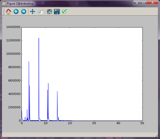
Fig. 1 Total ion chromatogram.

One drawback here is that you have to type these commands every time you want to see this plot. Alternatively, you can put all of these commands into a text file and run it with Python directly. Copy the following code into a plain text file called “tic_plot.py”. (See Working with Text Files for more information on making Python program files.) Note: It is common practice to do all imports at the top of a Python program. That way it is clear exactly what code is being brought into play.

import matplotlib.pyplot as plt
from gcmstools.filetypes import AiaFile

data = AiaFile('datasample1.CDF')
plt.plot(data.times, data.tic)
plt.show()

Run this new file using the python command from the terminal. The plot window will appear, and you can interact with the data. However, you will not be able to work in the terminal again until you close this window.

gcms>$ python tic_plot.py

Alternatively, you can run this program directly from IPython. This has the advantage that once the window is closed, you are dropped back into an IPython session that “remembers” all of the variables and imports from your program file. See Appendix A for more information here.

In : %run tic_plot.py

Working with multiple data sets

In the example above, we opened one dataset into a variable called data. If you want to manipulate more than one data set, the procedure is the same, except that you will need to use different variable names for your other data sets. (Again, using AiaFile importer as an example, but this is not required.)

In : data2 = AiaFile('datasample2.CDF')

These two data sets can be plot together on the same figure by doing the following:

In : plt.plot(data.times, data.tic)
Out:
[<matplotlib.lines.Line2D at 0x7f34>]

In: plt.plot(data2.times, data2.tic)
Out:
[<matplotlib.lines.Line2D at 0x02e3>]

In: plt.show()

The window shown in :num:`Figure #twotic` should now appear. (There is a blue and green line here that are a little hard to see in this picture. Zoom in on the plot to see the differences.)

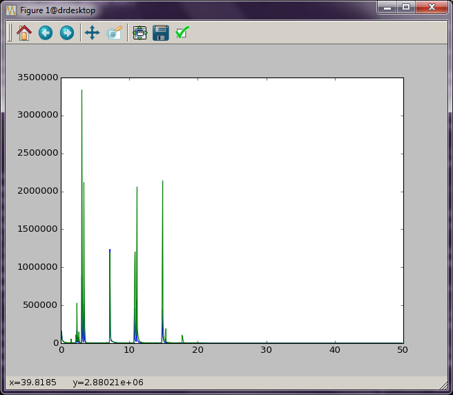
Fig. 2 Two TIC plotted together.