Referencing and Fitting
In order to properly integrate your GCMS data, you must assign reference information followed by running an appropriate fitting routine. This section discusses methods to accomplish this using gcmstools.
The general usage of the classes described in this section is identical. First, you will need one or more GCMS data objects, which you created in the previous section. Then you will create both reference and fitting object instances, which act as factories. You pass in a GcmsFile object, and the appropriate reference and fitting information will then be inserted into the object. Below is a pseudocode example that process:
# This will not work. See below for specific imports
In : from gcmstools.reference import FakeRef

In : from gcmstools.fitting import FakeFitter

In : ref = FakeRef('appropriate_reference_file')

In : fit = FakeFitter()

In : ref(data1)
Referencing: fakedata1

# Or pass in a list of many data objects
In : ref([data2, data3])
Referencing: fakedata2
Referencing: fakedata3

In : fit(data1)
Fitting: fakedata1

In : fit([data2, data3])
Fitting: fakedata2
Fitting: fakedata3

# all data sets now contain reference and fit information
Each reference and fitting type may append different types of information into your GCMS file object. In general, reference attributes will be preceded by “ref_”, whereas fitting attributes will be preceded by “fit_”.
One exception is that all referencing objects will add both a ref_cpds
list and a ref_meta dictionary to the GCMS data object. The former is a
list of the reference compound names that you define in the reference file,
called “appropriate_reference_file” in our example. (More on this file
below.) The latter contains metadata also extracted from the reference input
file. When you pass your GCMS data object into the fitting object, an
extracted integral will be added to that dictionary. These raw integrals are
not useful on their own, but are used in the Calibration and Concentration Determination section later
in this tutorial.
In : data1.ref_cpds
['ref_cpd_name1', 'ref_cpd_name2', 'ref_cpd_name3', ... ]

In : data1.ref_meta['ref_cpd_name1']['integral']
102237.01
Reference Files
In order to properly reference and fit your data set, you must prepare an appropriate reference input file. These files are simply plain text documents that describe the reference information for all of the compounds you would like to process. The structure of these files is very important. They are made up of a series of labels followed by the pertinent value. For example, all references must have a “NAME” label that provides the name of the reference compound. (It’s probably best if this is concise.) In addition, if you are going to be integrating this compound, then you must include “START” and “STOP” values, which are the starting and ending elution times for the integration region. (Don’t include the units.) Each reference compound must be separated by a blank line. Below is a truncated example for “benzene”:
NAME:benzene
START:2.9
STOP:3.5
Additional labels can be added if you’d like to include extra metadata about
your reference compound, such as retention index or molecular weight. For all
reference file types, lines starting with # are treated as comment lines
and ignored. This can be useful if you want to add some notes or to remove
reference information without deleting them entirely.
Each reference/fitting type works with different reference files, so see the sections below for specifics.
Non-negative Least Squares
Collecting References for NNLS
The non-negative least squares (NNLS) fitting routine can use two different reference files. There are examples of both in the sample data directory: “ref_spec.txt” and “ref_spec2.MSL”.
In : from gcmstools.general import get_sample_data

In : get_sample_data('ref_spec.txt')

In : get_sample_data('ref_spec2.MSL')
MSL files are typically autogenerated by external software, such as AMDIS or the NIST Spectral Database. The “txt” file was hand generated. In addition to the “NAME” (and potentially “START” and “STOP”) label, these files have a section that starts with the label “NUM PEAKS” and is followed by the m/z and intensity information for the reference compound. As the MSL file is autogenerated, you will most like not have to adjust these data. However, you will have to add these data into the “txt” file by hand.
The “NUM PEAKS” label in a “txt” file is followed by (at least) two space-separated columns of MS data. The first column must be the m/z values, and the second column contains the associated intensity values. Intensities are normalized on import, so it is not necessary to do this by hand.
Remember, each reference compound must be separated by a blank line. Below is a small sample of one a “txt” file. An MSL file would differ only in the format of the “NUM PEAKS” section.
NAME:benzene
START:2.9
STOP:3.5
NUM PEAKS:
  36 1.82 18
  37 6.5 65
  38 7.38 74
  39 15.17 152
  49 6.91 69
.
.
.
The online MS repository massBank is a useful place to find these m/z and intensity values. The data from that site is already formated correctly for this file type.
Loading Reference Spectra
There are two objects located in gcmstools.reference for loading these reference
data, TxtReference and MslReferece, which are used for “txt” and
MSL reference files, respectively. In this example, we’ll use
TxtReferece, but the MSL version behaves in the same manner. The variable
data refers to a GCMS file object that we created earlier.
In : from gcmstools.reference import TxtReference

In : ref = TxtReference('ref_specs.txt')

In : ref(data)
Referencing: datasample1.CDF

In : data.<tab>
data.filename     data.index        data.masses       data.ref_meta
data.filetype     data.ref_array    data.ref_type     data.tic
data.intensity    data.ref_cpds     data.times
Several new attributes have been added to our GCMS data object, all of which
are prefixed with “ref_”. Below is a short description of each. ref_meta
and ref_cpds are described above.
ref_array: A 2D Numpy array of the reference mass spectra. Shape(# of ref compounds, # of masses)
ref_type: The name of the reference object type that was used to generate this information. (In this example, this would be “TxtReference”.)
Fitting the data
A non-negative least squares fitting object, Nnls, is provided in the
gcmstools.fitting module. To apply this fitting, simply call
the fitting instance with a data object or list of data objects. This must be
done after the data has been passed through a reference object.
In : from gcmstools.fitting import Nnls

In : fit = Nnls()

In : fit(data)
Fitting: datasample1.CDF

In : data.<tab>
data.filename     data.tic          data.fit_sim      data.ref_cpds
data.filetype     data.index        data.intensity    data.ref_meta
data.fit_coef     data.fit_csum     data.masses       data.ref_type
data.fit_type     data.ref_array    data.times
Again, several new attributes describing the fit, all starting with “fit_”, have been added to our data set.
fit_type: A string that names the fitting object used to generate this data. (In this case, it would be “Nnls”.)
fit_coef: A 2D Numpy array of the least squares coefficients at every time point. They do not correspond to proper integrations, so they should be used with caution. An example using these values to simulate a MS spectrum is shown in Appendix B.
fit_sim: A 2D numpy array of simulated GCMS curves that were generated from the fit. Shape(# of time points, # of reference compounds)
fit_csum: A 2D numpy array that is the cumulative summation of fit_sim along the time axis, so it has the same shape as that array. An integral of a particular region can be obtained by determining the difference between any two points along the time dimension in this array. However, the calibration object automatically handles this integration, so you shouldn’t need to do integrations in this manner.
As stated above, the integrals for the reference compounds have also been
added to the ref_meta dictionaries.
Plotting the Fit
You can do a quick visual check of the fits using Matplotlib. More advanced examples are presented in Appendix B. The output of the commands below is shown in :num:`Figure #fitcheck`.
In : import matplotlib.pyplot as plt

In : plt.plot(data.times, data.tic, 'k-', lw=1.5)
Out: [<matplotlib.lines.Line2D at 0x7f9b2905df60>]

In : plt.plot(data.times, data.fit_sim)
Out:
[<matplotlib.lines.Line2D at 0x7f9b2f0df160>,
 <matplotlib.lines.Line2D at 0x7f9b29063ac8>,
 <matplotlib.lines.Line2D at 0x7f9b29063d30>,
 <matplotlib.lines.Line2D at 0x7f9b29063f98>,
 <matplotlib.lines.Line2D at 0x7f9b28fef240>,
 <matplotlib.lines.Line2D at 0x7f9b28fef4a8>,
 <matplotlib.lines.Line2D at 0x7f9b28fef710>,
 <matplotlib.lines.Line2D at 0x7f9b28faf720>]

In : plt.legend(["TIC",] + data.ref_cpds) # This isn't necessary
Out: <matplotlib.legend.Legend at 0x7f9b25a35438>

In : plt.show()
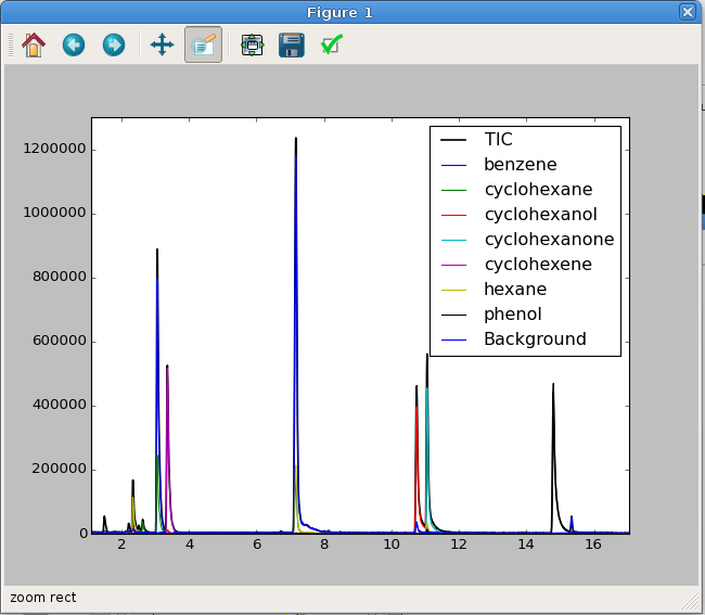
Fig. 3 An interactive plot of the TIC and the NNLS simulated fits. This has been zoomed in to highlight the fit and data.